Vol 2, Issue 8. Quarter 4 – 2025.

When I was a child back in the 1970’s I would often overhear my mother speaking on the phone and sometimes I would hear the word “SHARP”, as in “girl, that was a sharp outfit”, or “he sure is a sharp dresser.” The work Sharp meant stylish, cool, fashionable, etc. Because of that upbringing, I have always had an appreciation for things that are Sharp. Many years later I ran into something called the “Sharpe Ratio” and thought, “what the heck is that?” Well it turns out that both Sharp, and Sharpe still mean the same thing – just in different worlds. Allow me to explain.

William F. Sharpe received the Nobel prize in economics in 1990 for the Capital Asset Pricing Model (CAPM), but let’s not get too far ahead of ourselves. The CAPM can be developed using a simple idea. If we look at the ratio of expected investment returns and the variance of those returns we have a simple numerical value, and the higher this value the batter. This ratio became known as the Sharpe ratio and to coin a phrase the “Sharper the better.”

I like this idea because it can be explained in 2 dimensions, I can’t draw a picture in more than two dimensions, and the only reason that I can do that, is that Excel will do it for me. Specifically, the two dimensions are an Average, and a Standard Deviation. Since we will be speaking about Normally distributed variables, this is typically written as μ and σ.

An investment is a claim on future cash flows. When we purchase a financial asset (like a bond or a share of stock) we generally don’t know exactly what the associated cash flows will be. That fact is what we formally refer to as Risk. We can use history as a guide to come up with estimates about the parameters of those cash flows to figure out the Average Return and the Standard Deviation of those returns over some span of history and work with that. Note that there is a special case. A Risk-free bond is assumed to guarantee the cash flows. For such instruments, the variance of the returns is thus, 0.

You may ask “why do we need 2 dimensions at all?” A greater return is clear better than a lower return. The answer is that you are not “risk-neutral,” which simply means that you care about the risk. All that this means is that a smaller standard deviation is better than a larger one. Frankly, I do  not need to get into a deep discussion about why you think this way. I simply need to recognize that you do. How do I know this?  Consider 2 assets. The first will be labeled “Risk Free”. This asset has a positive expected return (μ_F) and a Standard Deviation of its return (σ_F) across history equal to 0. Let the other asset be labeled “Risky”. This one has an expected return that is greater than this risk free rate (μ_R > μ_F) and a Standard Deviation of those returns across history (σ_R > σ_F) which is greater than 0. If anyone were truly Risk-neutral they would always purchase the Risky asset. This means that if you have EVER purchased any asset that was risk-free, you are not Risk-Neutral. This just means that you are not a lunatic, because the risk matters to you to some degree. This has made our lives much more complex. I cannot simply look at the expected returns to make a decision. I must also consider the variance.

There is a silver lining in this story. I can look at the ratio of these things and reduce the focus to a single number. Specifically, the Sharpe ratio can be defined as S_r = E[R_r – R_f]/ σ_R. (What the hell did he just say?) The Sharpe ratio has 2 parts. The first part (E[μ_r – μ_f]) is the expected value of the return above the risk free rate. The subscript “r” refers to a risky asset like a share of stock. The subscript “f” refers to the risk free asset like a 30 day treasury bond. The second part of the equation (σ_R) is the standard deviation of the return on the risky asset. (Again, this assumes that the standard deviation on the return on the risk-free asset is 0, cause that’s what risk-free means.)

Here is the piece of insight that matters. If investment A has a higher Sharpe ratio than investment B, investment A is better! That’s about as straight-forward as I can make it. Let’s consider the 2 simplest cases.

Case 1: μ_A > μ_B and σ_A = σ_B. The expected return of asset A is greater and you are taking on the same amount of risk. This is a “no-brainer” choice. Notice that this does NOT mean that the realized outcome will always be better, but you can’t make the purchase decision based on that, because it doesn’t exist yet.

Case 2: μ_A = μ_B and σ_A < σ_B. Here the expected return is the same but one has a lower variance. The one with lower variance is better because you can count on that money. The landlord doesn’t want to hear, “there is a 50/50 chance that you get paid tomorrow”. All she wants to hear is “here is your money.”

More broadly, a higher standard deviation is bad for at least 3 reasons.

1. It makes holding the asset more painful. Seeing a value go down ain’t fun, even if you fully expect it to “come back” one day.
2. The inevitable drops that occasionally come with a higher variance give us less confidence in the outcome. With reduced confidence, you will run away whenever you get “scurred.”
3. Liquidity is reduced with variance. Something may go south in some other part of your life and you need your money TODAY. The presence of variance in your investment means there is some chance that you would then have to sell at a loss to fill that immediate need and that’s not good.

Now, let’s deal with the hard one.

Case 3: μ_A > μ_B and σ_A > σ_B. You have to expect this because Risk and Return go hand in hand. If an investment promises greater risk, you would never buy it unless it also included a higher return. This was the lesson from Case 2.

In this setting it is the ratio of the two elements that matters. To see this, consider the picture shown below. Point A relates to a share of common stock that historically had a Standard Deviation of 40% (about average for stocks in the S&P 500) but has shown an average return of 14%. Point B relates to the S&P 500 as a whole which has historically had a Standard Deviation of roughly 20% and an average return of 12%. These points stand in comparison to Point F, which reflects an assumed Risk Free rate of 4% and a standard deviation of 0%.  (Remember, for this discussion Risk-Free just means that variance is 0!) The slope of the line between Point F and Point A is lower than the slope of the line between Point F and Point B. In this case asset B is preferred over asset A. Notice that if the expected return on Asset A had been about 20%, it would have been preferred. In that case we would say the the expected return is high enough to compensate a risk-averse investor for the extra risk.

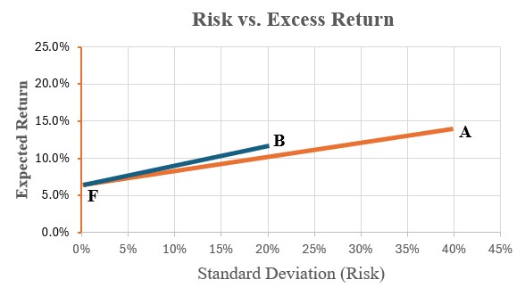
You will – no doubt – notice that the line from F to A is longer and you may wonder if this matters. The short answer is NO, that does not matter. This is true because I can use leverage (borrowing) to extend the line to point B to make it as long as the line to point A. This is why the slope is all that I need to know.

I recognize that this lesson was a little hard. Its not nearly as easy as simply focusing on a single factor like average return. That is unfortunate, but unavoidable. I understand the complaint that this is getting tricky, but if it were much easier than this, you’d already be rich. Here are a few, key take – aways.

1. Risk and reward go hand in hand, and you cannot make an investment decision without wrestling with both.
2. A bit of clever organization of the related information can make thinking about the tradeoff manageable.
3. If one insists on doing this oneself (AS I ALWAYS WILL) you are going to have to learn a bit of the language and run your own numbers.
4. We are here to walk with you as you do that.

Stay with us, and your inevitable wealth will follow. It may be slow, but it will be real.